Format Number in Thousand or Million

Thousand

#0.00,

Million

#0.00,,

1 comma stands for thousand.
2 commas stand for million.

0.00,, will convert numbers into million format by having leading 0 before decimal and 2 numbers are displayed after decimal. For example 100,000 will be displayed as 0.10. Format as 0.0,, will display 100,000 as 0.1.

The # symbol is a placeholder for optional digits. When a number has fewer digits than # symbols in the format, nothing will be displayed. For example, the custom format #.## will display 1.15 as 1.15 and 1.1 as 1.1 not 1.10.

Hide 0 Pivot Table Values or Show As Blank

Say you have a pivot table. You want to format the number:

1. In million for ∑ Values >0
2. Show blank for ∑ Values =0

Simply use below in Value Field Settings → Number Format → Custom and type:

#,##0.000,,;-0;;@

Example: Below 'LOS' values are equal to 0 but now appeared as blank

How To Group Percentages in Excel Pivot Table

Objective:

1. You have a column that contains percentage
2. Then you want to group the percentage by certain range. For example:
• By 10%: 1-10%, 11-20%, 21-30% and so on
• By 20%: 1-20%, 21-40%, 41-60% and so on
3. Insert 1 column and apply below formula linked to the percentage

Range of 10%:

TEXT(IF(A1<=0.1,0,CEILING(A1,0.1)*100-9),"0-")&TEXT(CEILING(A1,0.1),"0%")

Range of 20%:

TEXT(IF(A1<=0.2,0,CEILING(A1,0.2)*100-19),"0-")&TEXT(CEILING(A1,0.2),"0%")

The group is useful for you to summarize your data by using pivot table.

HowTo Hide Field Buttons in Pivot Chart

1. Assume you have a chart like below and you want to hide Field Buttons (the ones highlighted in red)

2. Click at the chart. Then go to Analyze → Field Buttons → select Hide All

3. Done! All the field buttons are now hidden

Advanced Filter

It is used to filter selected range but works differently from Filter command.

It displays the Advanced Filter dialog box instead of the AutoFilter menu.

You have to set the criteria to filter separately from the data range. You can put above your data or anywhere as long as outside from your data.

How to use:

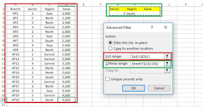
• Say you have a set of table like below in range A1:D21

• Type your criteria anywhere. You MUST specify each header that you want to filter and its value. Cells in yellow are the header title. Example as per below table. Criteria in range G1:I2.

• Sector = 3, Region = South and Sales = any value. Now go to Data → select Advanced in Sort & Filter.

• A dialog box will be displayed to ask for the range that you want to filter and criteria range for criteria that you want to filter. Just select the range accordingly and then click OK. Example as per below picture. Refer the box border color to differentiate between data range (red) and criteria range (green).

• Result as follow:

• You can also add more criteria like below. If you want to filter a column that contains number, you can use = for equal to, > for greater than, < for less than >= for greater than or equal to, <= for less than or equal to.

• Result as follow:

Hide Data in Selected Cells

Is easy to hide rows or columns by using hide or unhide feature in excel.

Have you ever tried to hide selected cells only? Maybe you used white font to make it invisible or font color equal to your background color.

Easy trick to hide values in selected cells is by changing the cell format function.

1. Choose the cells and go to Home → Font → Open Format Cells → Number Tab → Custom → Type ;;; → Click OK
2. Alternatively, select cells → right click → Format Cells... → Number → Custom → Type ;;; → OK

HowTo Select A Worksheet in A Workbook with Many Worksheets

Too many worksheets? Tired of using scroll left and right?

Too bad if you cannot reduce worksheets. It is best to have minimum worksheets as much as possible.

If you have to live with it, well, there is an alternative to speed up your works. Stop scrolling from now.

How To:

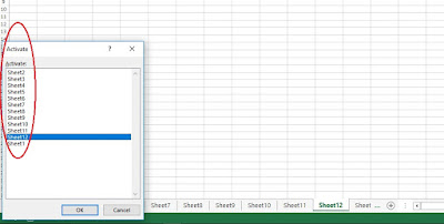
1. Right click at Excel ScrolBar (left side at triangle button)
2. Activate worksheet column will appear
3. Then select worksheet that you want
4. Done!

HowTo Select A Worksheet in A Workbook with Many Worksheets

HowTo Select A Worksheet in A Workbook with Many Worksheets

HowTo Print Comments in Excel

How To:

1. Goto Review → Show All Comments
2. Page Layout → Page Setup Tab → Click small arrow down
3. Sheet → Print → Comments → select "As displayed on sheet" from dropdown

HowTo Print Comments in Excel

HowTo Print Comments in Excel

HowTo Print Comments in Excel

HowTo Disable GetPivotData

GETPIVOTDATA is complicated. Very hard to understand the logic. I really hate GETPIVOTDATA. Good thing is that this can be disable.

How To:

1. Click at Pivot Table area
2. GoTo Analyze Ribbon
3. Under PivotTable field
4. Click Options
5. Untick Generate GetPivotData